6 Quarto

6.1 Quartoとは

Quartoによって本文とコードを一緒に扱うことができ，きれいなレポート，報告書，そして最終的には論文を執筆することができる．

以下の説明で基本的なことが理解できたら Quartoのページを確認するとよい．細かな設定をすることで自分好みの自分好みの出力が可能となる．

ファイルの拡張子は.qmdとなる．ある程度ファイルに入力したら，Renderをクリックして実行する（自動的にファイルは上書き保存される）．するとHTMLファイルが作成される．

ヒント

ブラウザではなくRStudioの画面内で結果を表示させたい場合は，Renderの右の設定からPreview in Viewer Paneを選択し，Renderをクリックして実行する．もとに戻したい場合はPreview in Windowを選択する．

6.2 YAML headerの設定

一番上の部分（YAML headerと呼ばれ，YAMLはプログラミング言語であり，設定ファイルの記述のためによく用いられている）はまずは次のように設定しておく．これによって結果がHTMLで出力される．今回はオプションは最小限にし，目次だけが表示される設定にしている．

---
title: "Intro Quarto"
author: "Sho Fujihara"
format:
  html:
    toc: true
---

なお「教育調査分析法（第1回）」という授業の配布資料では次のような設定にしている．

---
title: "教育調査分析法（第1回）"
author: "藤原翔"
format:
  html:
    toc: true
    embed-resources: true
    standalone: true
    scrollable: true
    number-sections: true
    page-layout: full
crossref:
  fig-title: Figure     # (default is "Figure")
  tbl-title: Table     # (default is "Table")
  title-delim: ":"     # (default is ":")
execute:
  cache: true
  warning: false
  message: false
  echo: false
date: "2023-05-10"
editor: source
---

6.3 セクション

セクションについては# セクション名（ハッシュ1つ）を使用する．サブセクションについては## サブセクション名（ハッシュ2つを）を使用する．サブサブセクションについては### サブサブセクション名（ハッシュ3つを）を使用する．

6.4 コメントアウト

通常のRのスクリプトで用いていた#は，qmdファイルの本文中で使用すると，セクションになってしまう．次のようにでコメントを囲めばよい．

<!-- 
ここにコメントを書く．
-->

6.5 箇条書き

箇条書きには-を用いる．

- 1つ目
- 2つ目
   - 2つ目の1つ目
   - 2つ目の2つ目
- 3つ目
   - 3つ目の1つ目 
   - 3つ目の2つ目

1つ目
2つ目
- 2つ目の1つ目
3つ目
- 3つ目の1つ目
- 3つ目の2つ目

6.6 数式

$\LaTeX$の記法によって美しい数式を書くこともできる．数式は$$で囲む．

$$Y = b_0 + b_1X$$

$$\bar x = \frac{1}{n}\sum_{i=1}^n x_i$$

\[Y = b_0 + b_1X\]

\[\bar x = \frac{1}{n}\sum_{i=1}^n x_i\]

6.7 コードチャンク

```{r}と```の間にRのスクリプトや他の設定について入力する．たとえば1 + 2を計算したければ次のようにする．

```{r}
1 + 2
```

すると次のような結果が示される．

1 + 2

[1] 3

結果だけを表示させたければ#| echo: falseをつける．#|によって

```{r}
#| echo: false
1 + 2
```

[1] 3

パッケージの呼び出しとデータの出力も同様に行う．

```{r}
# パッケージの呼び出し
library(tidyverse)
# データの表示
starwars
# 身長のヒストグラム
starwars |> ggplot(aes(x = height)) +
  geom_histogram()
```

すると次のように表示される．

# パッケージの呼び出し
library(tidyverse)

── Attaching core tidyverse packages ──────────────────────── tidyverse 2.0.0 ──
✔ dplyr     1.1.2     ✔ readr     2.1.4
✔ forcats   1.0.0     ✔ stringr   1.5.0
✔ ggplot2   3.4.2     ✔ tibble    3.2.1
✔ lubridate 1.9.2     ✔ tidyr     1.3.0
✔ purrr     1.0.1     
── Conflicts ────────────────────────────────────────── tidyverse_conflicts() ──
✖ dplyr::filter() masks stats::filter()
✖ dplyr::lag()    masks stats::lag()
ℹ Use the conflicted package (<http://conflicted.r-lib.org/>) to force all conflicts to become errors

# データの表示
starwars

# A tibble: 87 × 14
   name     height  mass hair_color skin_color eye_color birth_year sex   gender
   <chr>     <int> <dbl> <chr>      <chr>      <chr>          <dbl> <chr> <chr> 
 1 Luke Sk…    172    77 blond      fair       blue            19   male  mascu…
 2 C-3PO       167    75 <NA>       gold       yellow         112   none  mascu…
 3 R2-D2        96    32 <NA>       white, bl… red             33   none  mascu…
 4 Darth V…    202   136 none       white      yellow          41.9 male  mascu…
 5 Leia Or…    150    49 brown      light      brown           19   fema… femin…
 6 Owen La…    178   120 brown, gr… light      blue            52   male  mascu…
 7 Beru Wh…    165    75 brown      light      blue            47   fema… femin…
 8 R5-D4        97    32 <NA>       white, red red             NA   none  mascu…
 9 Biggs D…    183    84 black      light      brown           24   male  mascu…
10 Obi-Wan…    182    77 auburn, w… fair       blue-gray       57   male  mascu…
# ℹ 77 more rows
# ℹ 5 more variables: homeworld <chr>, species <chr>, films <list>,
#   vehicles <list>, starships <list>

# 身長のヒストグラム
starwars |> ggplot(aes(x = height)) +
  geom_histogram()

`stat_bin()` using `bins = 30`. Pick better value with `binwidth`.

Warning: Removed 6 rows containing non-finite values (`stat_bin()`).

6.8 2段組み

次のように2段にわけて表示することもできる．#| eval: falseと#| echo: falseを使って，入力と出力をわけて示している．

::: .column
::: {.column width="48%"}
**入力**

```{r}
#| eval: false
library(tidyverse)
library(here)
d <- read_csv(here("data","raw","u001.csv"))
d
```
:::


::: {.column width="48%"}
**出力**

```{r}
#| echo: false
library(tidyverse)
library(here)
d <- read_csv(here("data","raw","u001.csv"))
d
```
:::
:::

入力

library(tidyverse)
library(here)
d <- read_csv(here("data","raw","u001.csv"))
d

出力

here() starts at /Users/sf/GitHub/R4SS

Rows: 1000 Columns: 72
── Column specification ────────────────────────────────────────────────────────
Delimiter: ","
dbl (72): caseid, sex, ybirth, mbirth, ZQ03, JC_1, JC_41, ZQ08A, ZQ08B, ZQ08...

ℹ Use `spec()` to retrieve the full column specification for this data.
ℹ Specify the column types or set `show_col_types = FALSE` to quiet this message.

# A tibble: 1,000 × 72
   caseid   sex ybirth mbirth  ZQ03  JC_1 JC_41 ZQ08A ZQ08B ZQ08C ZQ08D ZQ08E
    <dbl> <dbl>  <dbl>  <dbl> <dbl> <dbl> <dbl> <dbl> <dbl> <dbl> <dbl> <dbl>
 1  10001     1   1976     10     1     2    12     4     1     3     4     4
 2  10002     1   1972      1     1     2     9     6     2     2     4     6
 3  10003     1   1975      4     1     2     9     6     6     6     3     6
 4  10004     2   1974     11     1     2     7     6     1     1     5     1
 5  10005     1   1978      1     2    10    88     6     2     2     4     1
 6  10006     1   1984      2     2    10    88     6     1     2     6     3
 7  10007     2   1976      6     1     2     8     6     4     1     5     1
 8  10008     1   1975      4     1     2     9     5     2     2     4     4
 9  10009     2   1985      9     1     3     5     1     1     1     4     1
10  10010     1   1972      2     1     2     8     6     1     2     5     6
# ℹ 990 more rows
# ℹ 60 more variables: ZQ08F <dbl>, ZQ08G <dbl>, ZQ08H <dbl>, ZQ11_A <dbl>,
#   ZQ11_B <dbl>, ZQ11_C <dbl>, ZQ11_D <dbl>, ZQ11_E <dbl>, ZQ11_F <dbl>,
#   ZQ11_G <dbl>, ZQ11_H <dbl>, ZQ11_I <dbl>, ZQ11_J <dbl>, ZQ11_K <dbl>,
#   ZQ11_L <dbl>, ZQ11_M <dbl>, ZQ11_N <dbl>, ZQ11_O <dbl>, ZQ12 <dbl>,
#   ZQ14_1A <dbl>, ZQ14_1B <dbl>, ZQ14_1C <dbl>, ZQ14_1D <dbl>, ZQ23A <dbl>,
#   ZQ23B <dbl>, ZQ23C <dbl>, ZQ23D <dbl>, ZQ24 <dbl>, ZQ25 <dbl>, …

::: .column
::: {.column width="48%"}
**図を描くためのスクリプト**

```{r}
#| eval: false
# 身長のヒストグラム
starwars |> ggplot(aes(x = height)) +
  geom_histogram()
```
:::

::: {.column width="48%"}
**図の出力**

```{r}
#| echo: false
#| label: fig-hist
#| fig-cap: 身長のヒストグラム
# 身長のヒストグラム
starwars |> ggplot(aes(x = height)) +
  geom_histogram()
```
:::
:::

@fig-hist は身長のヒストグラムである．

図を描くためのスクリプト

# 身長のヒストグラム
starwars |> ggplot(aes(x = height)) +
  geom_histogram()

図の出力

`stat_bin()` using `bins = 30`. Pick better value with `binwidth`.

Warning: Removed 6 rows containing non-finite values (`stat_bin()`).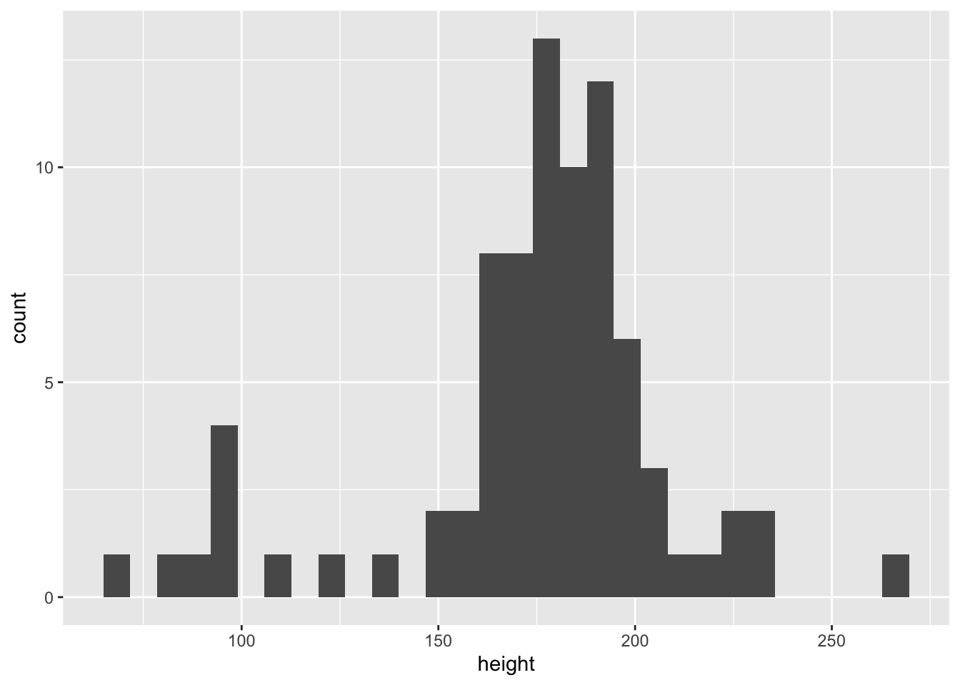

Figure 6.1 は身長のヒストグラムである．現在はFigure Xとなるように設定しているが，YAMLで変更可能である（図: Xや表: Xなど）．

6.9 パネルに分けて表示

:::{.panel-tabset}
## 入力

```{r}
#| eval: false
library(tidyverse)
library(here)
d <- read_csv(here("data","raw","u001.csv"))
d
```

## 出力

```{r}
#| echo: false
library(tidyverse)
library(here)
d <- read_csv(here("data","raw","u001.csv"))
d
```
:::

入力
出力

library(tidyverse)
library(here)
d <- read_csv(here("data","raw","u001.csv"))
d

Rows: 1000 Columns: 72
── Column specification ────────────────────────────────────────────────────────
Delimiter: ","
dbl (72): caseid, sex, ybirth, mbirth, ZQ03, JC_1, JC_41, ZQ08A, ZQ08B, ZQ08...

ℹ Use `spec()` to retrieve the full column specification for this data.
ℹ Specify the column types or set `show_col_types = FALSE` to quiet this message.

# A tibble: 1,000 × 72
   caseid   sex ybirth mbirth  ZQ03  JC_1 JC_41 ZQ08A ZQ08B ZQ08C ZQ08D ZQ08E
    <dbl> <dbl>  <dbl>  <dbl> <dbl> <dbl> <dbl> <dbl> <dbl> <dbl> <dbl> <dbl>
 1  10001     1   1976     10     1     2    12     4     1     3     4     4
 2  10002     1   1972      1     1     2     9     6     2     2     4     6
 3  10003     1   1975      4     1     2     9     6     6     6     3     6
 4  10004     2   1974     11     1     2     7     6     1     1     5     1
 5  10005     1   1978      1     2    10    88     6     2     2     4     1
 6  10006     1   1984      2     2    10    88     6     1     2     6     3
 7  10007     2   1976      6     1     2     8     6     4     1     5     1
 8  10008     1   1975      4     1     2     9     5     2     2     4     4
 9  10009     2   1985      9     1     3     5     1     1     1     4     1
10  10010     1   1972      2     1     2     8     6     1     2     5     6
# ℹ 990 more rows
# ℹ 60 more variables: ZQ08F <dbl>, ZQ08G <dbl>, ZQ08H <dbl>, ZQ11_A <dbl>,
#   ZQ11_B <dbl>, ZQ11_C <dbl>, ZQ11_D <dbl>, ZQ11_E <dbl>, ZQ11_F <dbl>,
#   ZQ11_G <dbl>, ZQ11_H <dbl>, ZQ11_I <dbl>, ZQ11_J <dbl>, ZQ11_K <dbl>,
#   ZQ11_L <dbl>, ZQ11_M <dbl>, ZQ11_N <dbl>, ZQ11_O <dbl>, ZQ12 <dbl>,
#   ZQ14_1A <dbl>, ZQ14_1B <dbl>, ZQ14_1C <dbl>, ZQ14_1D <dbl>, ZQ23A <dbl>,
#   ZQ23B <dbl>, ZQ23C <dbl>, ZQ23D <dbl>, ZQ24 <dbl>, ZQ25 <dbl>, …

6.10 参考文献

Zoteroなどの文献管理アプリを通じてbibファイルを作成し，引用する．

@knuth84とすれば Knuth (1984) となる． [@knuth84]とすれば (Knuth 1984) となる．