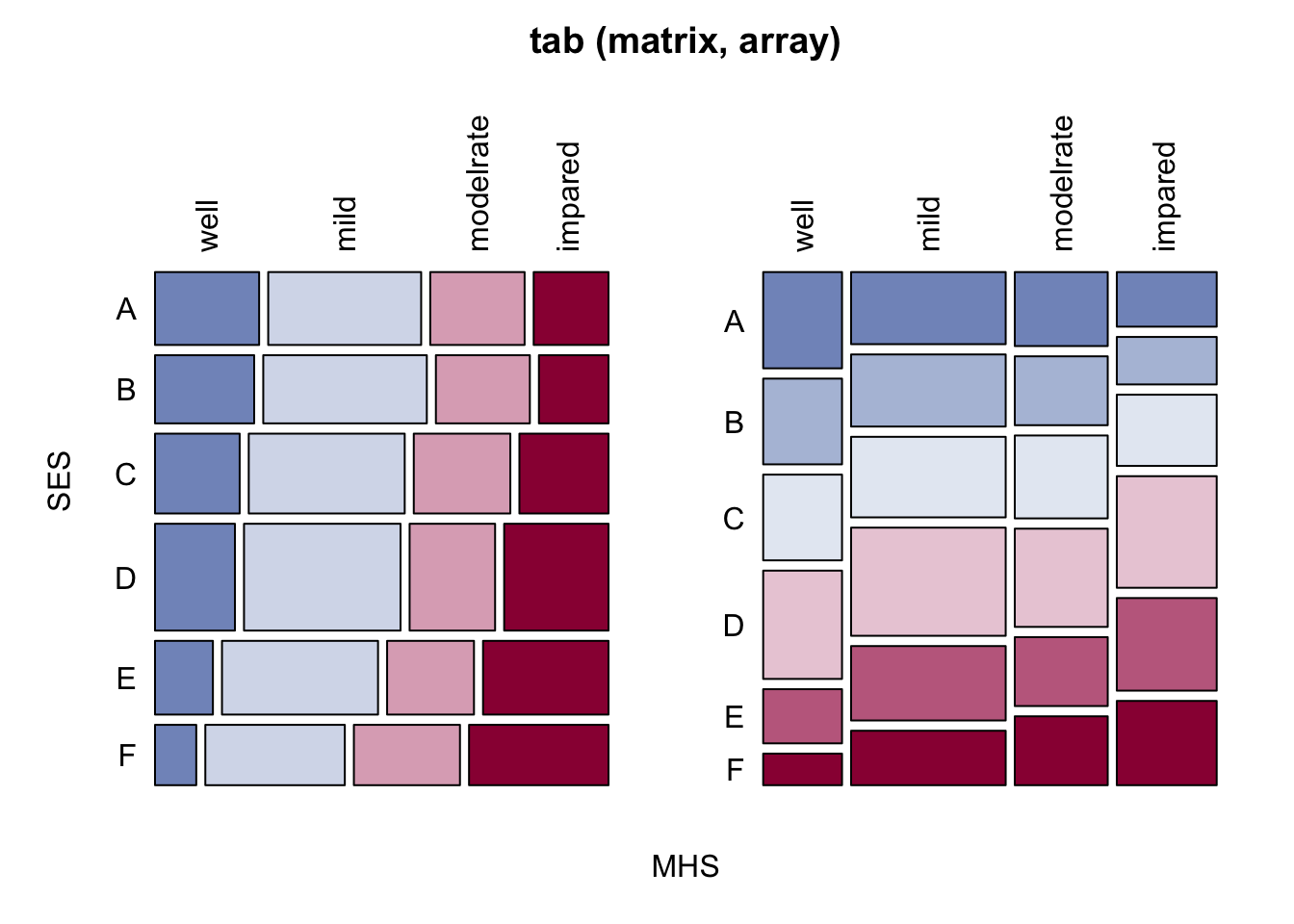
1 第1章

本章ですこし触れられてる連関の尺度のいくつかはDescToolsパッケージのAssocsで求めることができる．
「シリーズ編者による内容紹介」の精神的健康と親の社会経済的地位（SES）に関するミッドタウン・マンハッタンデータ（the Midtown Manhattan data）を用いて分析する．

# 元データの入力（xページ）
Freq <- c( 64,  94, 58, 46,
           57,  94, 54, 40,
           57, 105, 65, 60,
           72, 141, 77, 94,
           36,  97, 54, 78,
           21,  71, 54, 71)

# データを表形式に変換
tab <- matrix(
  Freq,
  nrow = 6,
  ncol = 4,
  byrow = TRUE,
  dimnames = list(
    SES = LETTERS[1:6],
    MHS = c("well",
            "mild",
            "moderate",
            "impaired")
  )
)
tab

   MHS
SES well mild moderate impaired
  A   64   94       58       46
  B   57   94       54       40
  C   57  105       65       60
  D   72  141       77       94
  E   36   97       54       78
  F   21   71       54       71

DescToolsパッケージを用いる．

library(DescTools)
DescTools::Desc(tab)

────────────────────────────────────────────────────────────────────────────── 
tab (matrix, array)

Summary: 
n: 1'660, rows: 6, columns: 4

Pearson's Chi-squared test:
  X-squared = 45.985, df = 15, p-value = 5.346e-05
Log likelihood ratio (G-test) test of independence:
  G = 47.418, X-squared df = 15, p-value = 3.155e-05
Mantel-Haenszel Chi-squared:
  X-squared = 37.156, df = 1, p-value = 1.091e-09

Contingency Coeff.     0.164
Cramer's V             0.096
Kendall Tau-b          0.120

                                                      
      MHS     well   mild   moderate   impaired    Sum
SES                                                   
                                                      
A     freq      64     94         58         46    262
      perc    3.9%   5.7%       3.5%       2.8%  15.8%
      p.row  24.4%  35.9%      22.1%      17.6%      .
      p.col  20.8%  15.6%      16.0%      11.8%      .
                                                      
B     freq      57     94         54         40    245
      perc    3.4%   5.7%       3.3%       2.4%  14.8%
      p.row  23.3%  38.4%      22.0%      16.3%      .
      p.col  18.6%  15.6%      14.9%      10.3%      .
                                                      
C     freq      57    105         65         60    287
      perc    3.4%   6.3%       3.9%       3.6%  17.3%
      p.row  19.9%  36.6%      22.6%      20.9%      .
      p.col  18.6%  17.4%      18.0%      15.4%      .
                                                      
D     freq      72    141         77         94    384
      perc    4.3%   8.5%       4.6%       5.7%  23.1%
      p.row  18.8%  36.7%      20.1%      24.5%      .
      p.col  23.5%  23.4%      21.3%      24.2%      .
                                                      
E     freq      36     97         54         78    265
      perc    2.2%   5.8%       3.3%       4.7%  16.0%
      p.row  13.6%  36.6%      20.4%      29.4%      .
      p.col  11.7%  16.1%      14.9%      20.1%      .
                                                      
F     freq      21     71         54         71    217
      perc    1.3%   4.3%       3.3%       4.3%  13.1%
      p.row   9.7%  32.7%      24.9%      32.7%      .
      p.col   6.8%  11.8%      14.9%      18.3%      .
                                                      
Sum   freq     307    602        362        389  1'660
      perc   18.5%  36.3%      21.8%      23.4% 100.0%
      p.row      .      .          .          .      .
      p.col      .      .          .          .      .

DescTools::Assocs(tab)

                       estimate  lwr.ci  upr.ci
Contingency Coeff.       0.1642       -       -
Cramer V                 0.0961  0.0482  0.1102
Kendall Tau-b            0.1202  0.0822  0.1583
Goodman Kruskal Gamma    0.1543  0.1056  0.2029
Stuart Tau-c             0.1247  0.0852  0.1643
Somers D C|R             0.1131  0.0773  0.1489
Somers D R|C             0.1278  0.0873  0.1684
Pearson Correlation      0.1497  0.1023  0.1964
Spearman Correlation     0.1485  0.1011  0.1952
Lambda C|R               0.0000  0.0000  0.0000
Lambda R|C               0.0000  0.0000  0.0000
Lambda sym               0.0000  0.0000  0.0000
Uncertainty Coeff. C|R   0.0106  0.0047  0.0164
Uncertainty Coeff. R|C   0.0080  0.0036  0.0125
Uncertainty Coeff. sym   0.0091  0.0041  0.0142
Mutual Information       0.0206       -       -

次のように個別に尺度を求めることもできる．詳しくは?DescToolsのStatistics:を確認してほしい．

DescTools::CramerV(tab, conf.level = 0.95)

  Cramer V     lwr.ci     upr.ci 
0.09609364 0.04817087 0.11017098

DescTools::Lambda(tab, conf.level = 0.95)

lambda lwr.ci upr.ci 
     0      0      0

DescTools::GoodmanKruskalTau(tab, conf.level = 0.95)

       tauA      lwr.ci      upr.ci 
0.004913157 0.002173427 0.007652887

DescTools::KendallTauB(tab, conf.level = 0.95)

     tau_b     lwr.ci     upr.ci 
0.12023215 0.08217305 0.15829125

DescTools::StuartTauC(tab, conf.level = 0.95)

      tauc     lwr.ci     upr.ci 
0.12473799 0.08520269 0.16427329

DescTools::GoodmanKruskalGamma(tab, conf.level = 0.95)

    gamma    lwr.ci    upr.ci 
0.1542894 0.1056412 0.2029376

DescTools::SomersDelta(tab, conf.level = 0.95)

    somers     lwr.ci     upr.ci 
0.12783809 0.08727872 0.16839747

DescTools::UncertCoef(tab, conf.level = 0.95)

         uc      lwr.ci      upr.ci 
0.009135369 0.004068778 0.014201959

1.1 クラメールのV

クラメールの$V$も連関の強さをみる指標であり，次のように定義される．

\[\begin{equation} V = \sqrt{\frac{\chi^2/n}{{\rm min}(I-1,J-1)}} \end{equation}\]

${\rm min}(I-1,J-1)$は括弧内の最小の値であり，${\rm min}(I,J)-1$と考えても良い．値の取りうる範囲は\[0 \leq V \leq 1\]となり，値が大きいほど2つの変数の連関は強いといえる．

ではクラメールのVを自分で求めてみよう．chisq.test(tab)$statisticでカイ2乗値を取り出すことができるが，名前がついているのでunname関数で取り除く．as.numericとしても取り除くことができる．

tab

   MHS
SES well mild moderate impaired
  A   64   94       58       46
  B   57   94       54       40
  C   57  105       65       60
  D   72  141       77       94
  E   36   97       54       78
  F   21   71       54       71

X2 <- chisq.test(tab)$statistic |> unname()   # あるいはas.numeric()
V <- sqrt(X2/sum(tab)/(min(dim(tab)) - 1))
V

[1] 0.09609364

tabの2行目を10倍，1列目を10倍したデータを考える．これをtab10とする．

tab10 <- tab
tab10[,1] <- tab10[,1]*10
tab10[2,] <- tab10[2,]*10
tab

   MHS
SES well mild moderate impaired
  A   64   94       58       46
  B   57   94       54       40
  C   57  105       65       60
  D   72  141       77       94
  E   36   97       54       78
  F   21   71       54       71

tab10

   MHS
SES well mild moderate impaired
  A  640   94       58       46
  B 5700  940      540      400
  C  570  105       65       60
  D  720  141       77       94
  E  360   97       54       78
  F  210   71       54       71

この2つの表について先程の連関係数の値を確認すると，すべての係数について表によって値が異なる．

DescTools::CramerV(tab)

[1] 0.09609364

DescTools::CramerV(tab10)

[1] 0.08200758

DescTools::GoodmanKruskalTau(tab)

[1] 0.004913157

DescTools::GoodmanKruskalTau(tab10)

[1] 0.00498861

DescTools::KendallTauB(tab)

[1] 0.1202322

DescTools::KendallTauB(tab10)

[1] 0.0933437

DescTools::StuartTauC(tab)

[1] 0.124738

DescTools::StuartTauC(tab10)

[1] 0.05978172

DescTools::GoodmanKruskalGamma(tab)

[1] 0.1542894

DescTools::GoodmanKruskalGamma(tab10)

[1] 0.1840237

DescTools::SomersDelta(tab)

[1] 0.1278381

DescTools::SomersDelta(tab10)

[1] 0.1015444

DescTools::UncertCoef(tab)

[1] 0.009135369

DescTools::UncertCoef(tab10)

[1] 0.008655116

オッズ比に基づく尺度では表によって値は異ならない． Bouchet-Valat (2022) や Zhou (2015) を参照．

# 2つの表をマージしたデータも作成
tab_merge <- dplyr::bind_rows(data.frame(as.table(tab)),
                       data.frame(as.table(tab10)),
         .id = "Tab") |> 
  xtabs(Freq ~ SES + MHS + Tab, data = _)
tab_merge

, , Tab = 1

   MHS
SES well mild moderate impaired
  A   64   94       58       46
  B   57   94       54       40
  C   57  105       65       60
  D   72  141       77       94
  E   36   97       54       78
  F   21   71       54       71

, , Tab = 2

   MHS
SES well mild moderate impaired
  A  640   94       58       46
  B 5700  940      540      400
  C  570  105       65       60
  D  720  141       77       94
  E  360   97       54       78
  F  210   71       54       71

# intrinsic association coefficient
logmult::iac(tab, weighting = "none")

[1] 1.022284

logmult::iac(tab10, weighting = "none")

[1] 1.022284

logmult::iac(tab_merge, weighting = "none")

       1        2 
1.022284 1.022284

# Altham index
logmult::iac(tab, weighting = "none") * sqrt(nrow(tab) * ncol(tab)) * 2

[1] 10.01629

logmult::iac(tab10, weighting = "none") * sqrt(nrow(tab) * ncol(tab)) * 2

[1] 10.01629

logmult::iac(tab_merge, weighting = "none") * sqrt(nrow(tab) * ncol(tab)) * 2

       1        2 
10.01629 10.01629

# Shrinkage Estimation
logmult::iac(tab_merge, 
             weighting = "none", 
             shrink=TRUE) * sqrt(nrow(tab_merge) * ncol(tab_merge)) * 2 * 2

       1        2 
20.03259 20.03259

# Mean absolute odds ratio
logmult::maor(tab, weighting = "uniform")

[1] 1.695377

logmult::maor(tab10, weighting = "uniform")

[1] 1.695377

logmult::maor(tab_merge, weighting = "uniform")

       1        2 
1.695377 1.695377

ただし周辺重み付けをすれば値は異なる場合もある．

# intrinsic association coefficient
logmult::iac(tab, weighting = "marginal")

[1] 0.1773414

logmult::iac(tab10, weighting = "marginal")

[1] 0.1182336

# Mean absolute odds ratio
logmult::maor(tab, weighting = "marginal")

[1] 1.577478

logmult::maor(tab10, weighting = "marginal")

[1] 1.636068

練習問題

occupationalStatusはRの組み込みデータセットで、イギリス男性の父親（origin）と息子（destination）の職業地位（8段階）をクロス表にしたものである。

出典: Goodman (1979) Table 3.

occupationalStatus

      destination
origin   1   2   3   4   5   6   7   8
     1  50  19  26   8   7  11   6   2
     2  16  40  34  18  11  20   8   3
     3  12  35  65  66  35  88  23  21
     4  11  20  58 110  40 183  64  32
     5   2   8  12  23  25  46  28  12
     6  12  28 102 162  90 554 230 177
     7   0   6  19  40  21 158 143  71
     8   0   3  14  32  15 126  91 106

このデータを用いて、本章で紹介した連関の尺度（クラメールのV、Kendallの$\tau_b$、Goodman-Kruskalの$\gamma$、iac、maorなど）を計算し、結果を比較せよ。

参考文献

Bouchet-Valat, Milan. 2022. “General Marginal-free Association Indices for Contingency Tables: From the Altham Index to the Intrinsic Association Coefficient.” Sociological Methods & Research 51 (1): 203–36. https://doi.org/10.1177/0049124119852389.

Goodman, Leo A. 1979. “Simple Models for the Analysis of Association in Cross-Classifications Having Ordered Categories.” Journal of the American Statistical Association 74 (367): 537–52.

Zhou, Xiang. 2015. “Shrinkage Estimation of Log-odds Ratios for Comparing Mobility Tables.” Sociological Methodology 45 (1): 320–56. https://doi.org/10.1177/0081175015570097.